Milvus Architecture Explained: How a Distributed Vector Database Works

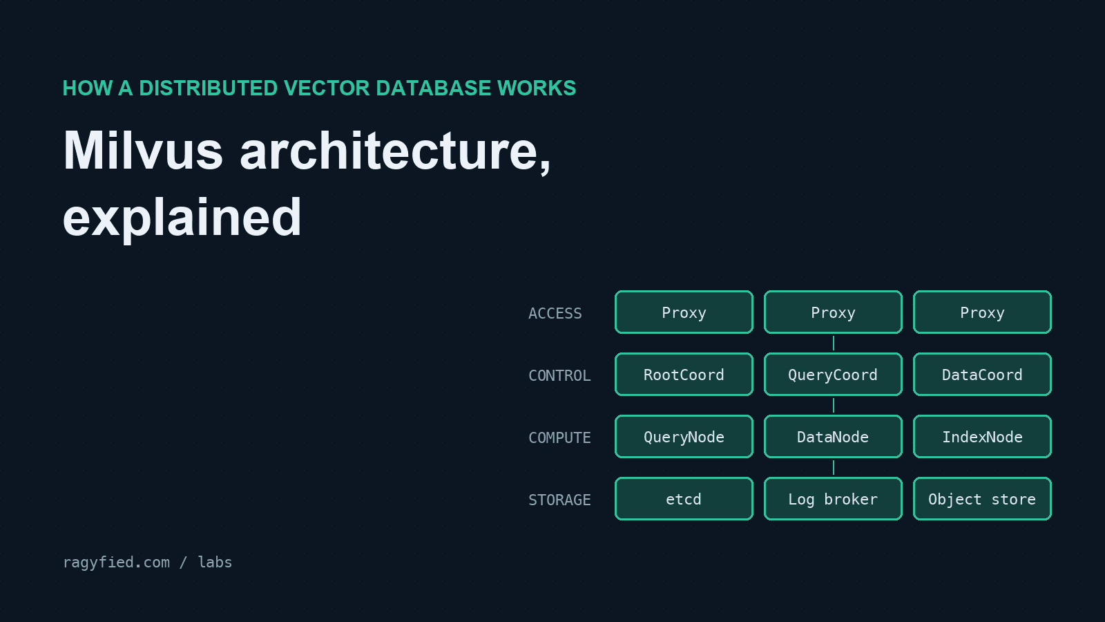
Most RAG tutorials treat the vector database as a box: put embeddings in, get neighbours out. That works until you have hundreds of millions of vectors, a freshness SLO and a pager. At that point the inside of the box matters, because its design decides what you can scale, what fails together and why your dashboards look the way they do.

Milvus is a good system to learn this from. It is open source, its architecture is documented in detail, and it takes the "separate everything" approach further than most. This post walks through the Milvus 2.5 architecture, the write path and the read path. If you'd rather click through it, the Milvus Architecture Lab has an interactive cluster map and animated request flows.

Four layers

Milvus splits the database into four layers, and only the bottom one holds state that must survive a failure.

1. Access layer: Proxies. Clients talk to a pool of stateless Proxies behind a load balancer. A Proxy validates requests against the cached schema, routes writes to the right shard, sends searches to the right query nodes, and merges partial results. Because Proxies hold no durable state, you can add or replace them freely.

2. Control plane: coordinators.

• RootCoord owns the catalog (collections, schemas, access control) and hands out IDs and logical timestamps. Those timestamps give every worker a shared order of operations.
• QueryCoord decides which QueryNode loads which segments and channels, keeps replicas placed and balanced, and manages the handoff from fresh data to indexed data.
• DataCoord manages the segment lifecycle: allocating segments, scheduling flushes, compaction and index builds.

Coordinators assign work; they never execute it. Coordinator high availability is active/standby, so a standby speeds up failover but adds no throughput.

3. Worker nodes, split by job.

• QueryNodes hold loaded segments in memory and run searches.
• DataNodes consume the write stream and persist it as segment files (binlogs), and they run compaction.
• IndexNodes build ANN indexes from sealed segments.

Each pool scales independently. An index-build backlog needs IndexNodes, not QueryNodes.

4. Durable dependencies.

• etcd stores metadata and service registrations with strong consistency.
• A log broker (Kafka or Pulsar in 2.5) holds the ordered stream of mutations.
• Object storage (S3, MinIO or compatible) holds segment data and index files.

This is the key idea: storage outlives workers. A replacement QueryNode loads its assigned segments from object storage and replays recent changes from the log. Nothing on the worker's local disk is the only copy.

The write path: log first

An insert never goes straight into an index.

1. Validate and order. The Proxy checks the rows against the schema, picks a shard, and gets timestamps and a segment allocation from the coordinators (batched, not one round trip per row).
2. Persist the log. The Proxy publishes the rows to the shard's channel in the log broker. Now the insert is acknowledged.
3. Consume in parallel. Two different consumers read that channel independently. DataNodes buffer the rows and flush them to object storage. QueryNodes add them to an in-memory growing segment, so recent data is searchable before it's indexed.
4. Seal, index, hand off. When a segment is sealed and flushed, DataCoord schedules an index build, an IndexNode writes the index files to object storage, and QueryCoord has the QueryNodes load the indexed segment in place of the growing data.

So an insert passes several milestones: acknowledged, searchable, flushed and indexed, each owned by a different component. When someone says "I inserted it but search can't find it", the question is which milestone it hasn't reached yet.

The read path: scatter, wait, merge

A search carries a query vector, an optional filter, top-k and a consistency level.

1. The Proxy sends the search to the shard leaders in one loaded replica. Replicas add throughput and availability; not every replica sees every request.
2. Each QueryNode compares how far it has consumed the log with the timestamp the consistency level requires. With Strong consistency it may wait for the stream to catch up. Bounded, the default, tolerates a small lag, and Eventually doesn't wait.
3. Workers search sealed (indexed) and growing segments in parallel and apply filters.
4. The Proxy merges each shard's top-k into the global top-k.

The practical consequence: search latency can be time spent waiting for freshness, not computing distances. That matters a lot when inserts and searches share a cluster, which the incident patterns show in detail.

Nodes vs replicas

Two scaling controls look alike but do different things:

• Adding QueryNodes spreads the segments of one loaded copy across more machines, so each holds less.
• Adding collection replicas creates another complete loaded copy, which needs its own group of QueryNodes.

A collection that needs 60 GB resident, with two replicas, needs 120 GB of QueryNode memory before headroom for growing data and recovery. The vector database sizing calculator does this arithmetic, and the scaling lab shows how replica groups break when you remove one node too many.

What this design means in production

The architecture predicts where Milvus clusters actually struggle:

• The write stream loads the query layer. QueryNodes consume inserts to keep fresh data searchable, so a bulk load can slow searches even when search traffic is flat.
• The broker is on every path. If Kafka or Pulsar throttles, persistence, freshness and eventually write admission all suffer.
• Metadata is a shared, non-sharded budget. Every collection, partition and segment adds keys in etcd, and every etcd member holds the full keyspace. Per-tenant collections hit this limit long before QueryNodes run out of memory.
• Long-lived gRPC connections defeat connection-level load balancing, so one Proxy can run hot while the fleet average looks healthy.

The follow-up posts cover two of these in depth: why etcd keeps growing and what compaction and defrag really do, and why inserts slow down Milvus search.

Going further

• The Milvus Architecture Lab has the interactive cluster map, animated flows, segment lifecycle, scaling models and incident patterns.
• The vendor-neutral version of these ideas is in the GenAI System Design course: Case Study: Inside a Distributed Vector Database.
• Newer Milvus releases replace parts of this design with a Streaming Node architecture. Everything above describes 2.5, so check the official docs for your version.